eBay-shipping-predictions
Predicting eBay Delivery Times
Millie Mince, Meghna Lohia, Hannah Mandell, Nate Dailey, and Indiana Huey
Abstract
In this project, we created and tuned models to predict delivery times for eBay packages given a dataset of eBay shipment records. We implemented four models—linear regression, fully connected neural network, XGBoost, and CatBoost—and compared the their effectiveness on the shipment data. We additionally examined different strategies to clean our dataset, engineer new features, and fine-tune each model. Ultimately, the fully connected model performed the best.
Introduction
The economy of online shopping is bigger than it has ever been and continues to grow each year. It follows that the market for being able to deliver goods quickly and reliably is becoming more and more competitive. In addition to improving the overall flow of transactions, knowing when a package will be delivered is a major factor in customer satisfaction, making the ability to accurately predict delivery dates essential to companies such as eBay.
The process of achieving this, however, poses many challenges. In the case of eBay, the majority of transactions are carried out between individual sellers and buyers, often resulting in the data for goods and their delivery being inconsistently recorded. This, in addition to packages being processed by a variety of different delivery services, means that data labels are frequently missing or incorrect. Further, the shipment date is largely left to the sole decision of each individual seller, resulting in a high degree of variability.
We worked to provide a solution to these problems and provide a model to enable the accurate prediction of delivery dates using machine learning.
To implement our model, a number of decisions were made and tested, including deciding the optimal means by which to clean the data (for instance, whether to omit training data that has missing or incorrect features or to assign it average values based on correctly labeled training data), deciding whether to compute the estimation holistically from shipment to delivery date or to compute multiple separate estimates on separate legs of the delivery process, and deciding which features to include and in which leg.
Should our model have some error, it is important that it produces random rather than systematic error. Specifically, we want to avoid creating a model which might consistently predict early delivery dates, which could lead to sellers and delivery services rushing packages and resulting in the employment of more non-sustainable methods, such as shipping half-full boxes, as well as increasing the pressure on employees to have to work faster and faster.
Using a loss function of the weighted average absolute error of the delivery predictions in days that was provided by eBay, our model achieved a loss of 0.411 where a loss of 0.759 was the baseline of random guessing.
Literature Review
The current state of research for the delivery time estimation problem shows how varied and nuanced delivery data and time estimation can be. There have been studies that focus on solving complex delivery problems such as having multiple legs of shipment, but also studies that are smaller in scale and detail how delivery time estimation is calculated for food delivery services. In this section, we will describe the relevant studies that cover delivery time estimation and discuss how each of their findings are applicable to our project.
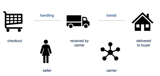
To solve a problem that is similar to ours, logistics supplier Aramex uses machine learning to predict delivery times, claiming that its model has increased the accuracy of delivery predictions by 74%. They describe a multi-leg approach in which the shipping process is divided into multiple steps to be estimated individually. For instance, the time from seller to processing hub is estimated separately from the time from customs to buyer in international transactions. The architecture integrates systems such as Amazon Redshift clustering and Amazon SageMaker to process its data. For our project, we also explore the benefits of splitting the different legs of shipment into smaller segments; handling time and shipment time.
Another study, Predicting Package Delivery Time For Motorcycles In Nairobi details how modifying the input variables for the model can help the model narrow in on important features. This study uses XGBoost, a supervised regression model, to predict the estimated time of delivery of a motorcycle-transported delivery in Nairobi. The researchers used input variables such as the client’s past orders information, the rider’s past orders information, weather, delivery distance, drop off and pickup location, and time of day. It describes the author’s approach to determining feature importance, particularly through graphics and XGBoost tree visuals. There is also a discussion of examining the results through the specific lens of a delivery date – it is better to predict late than early – and thus an optimized model should account for this by reprimanding a model harsher for predicting an early time, as opposed to a late time. We are using XGBoost as well because of its ability to determine feature importance when given a complex set of input variables.
Although it is a slightly modified problem, the researchers Araujo and Etemad (2020) document how they went about solving the problem of last-mile parcel delivery time estimation using data from Canada Post, the main postal service in Canada. They formalize the problem as an Origin-Destination Travel Time Estimation problem and compare several neural networks in order to generate the best results. Their findings indicate that a ResnNet with 8 residual convolutional blocks has the best performance, but they also explore VGG and Multi-Layer Perceptron models. We used the findings from this model to guide our choices when experimenting with different models.
Another version of the delivery time estimation problem is predicting workload (called WLC, workload control) and can be applied to predicting the delivery date in manufacturing plants. A paper by Romagnoli and Zammori (2019) describes how researchers set out to design a neural network that could streamline workload order (in order to minimize queues and optimize delivery dates). Their neural network had the following structure: an input layer with 12 inputs, a single output neuron delegated to make the forecast of the final delivery time, three hidden layers, each one with 32 neurons (plus a bias) with the Relu activation function, and batch normalization after each hidden layer. The authors found significant optimizations of manufacturing logistics and delivery times with their model. Initial trials to solve our problem used a neural network with a similar model, but we also modified the number of layers, inputs, and neurons to explore different structural possibilities.
Finally, there are numerous challenging elements that must be considered when solving this problem, and Wu, F., and Wu, L., (2019) cover the many difficulties of predicting package delivery time such as multiple destinations, time variant delivery status, and time invariant delivery features. Their article describes how DeepETA, their proposed framework, is a spatial-temporal sequential neural network model that uses a latest route encoder to include the location of packages and frequent pattern encoder to include historical data. There are 3 different layers to this model and through experimenting on real logistics data, the authors show that their proposed method outperforms start of the art methods. This paper is useful in identifying the challenges of predicting delivery time and how we may go about solving them.
Methods
Overview
To create our neural network model and attain our results, we used a number of tools for the different stages of our project. To construct our model, we used Pytorch, sklearn, and Jupyter notebooks for most of our development. We ran our code on the Pomona High Performance Computing servers to utilize more GPU power. We used a linear regression model with regularization penalties, as well as XGBoost, to infer which features were the most important for predicting (a) the handling time, and (b) the shipment time. We also compared our findings to a fully connected network. Finally, we used CatBoost to identify the hyperparameters to fine tune for our final model. Ultimately, we used CatBoost for our final predictions as it outperformed the other models.
Dataset
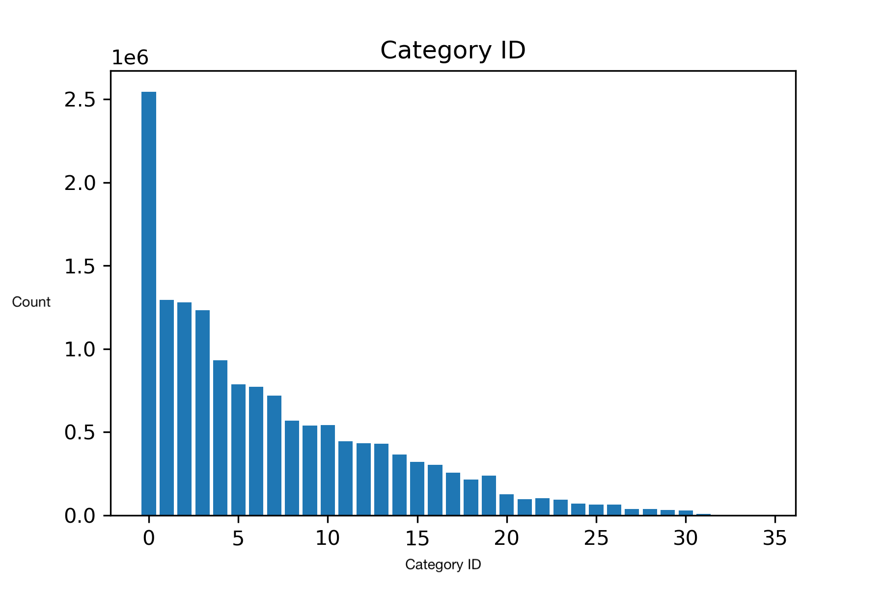
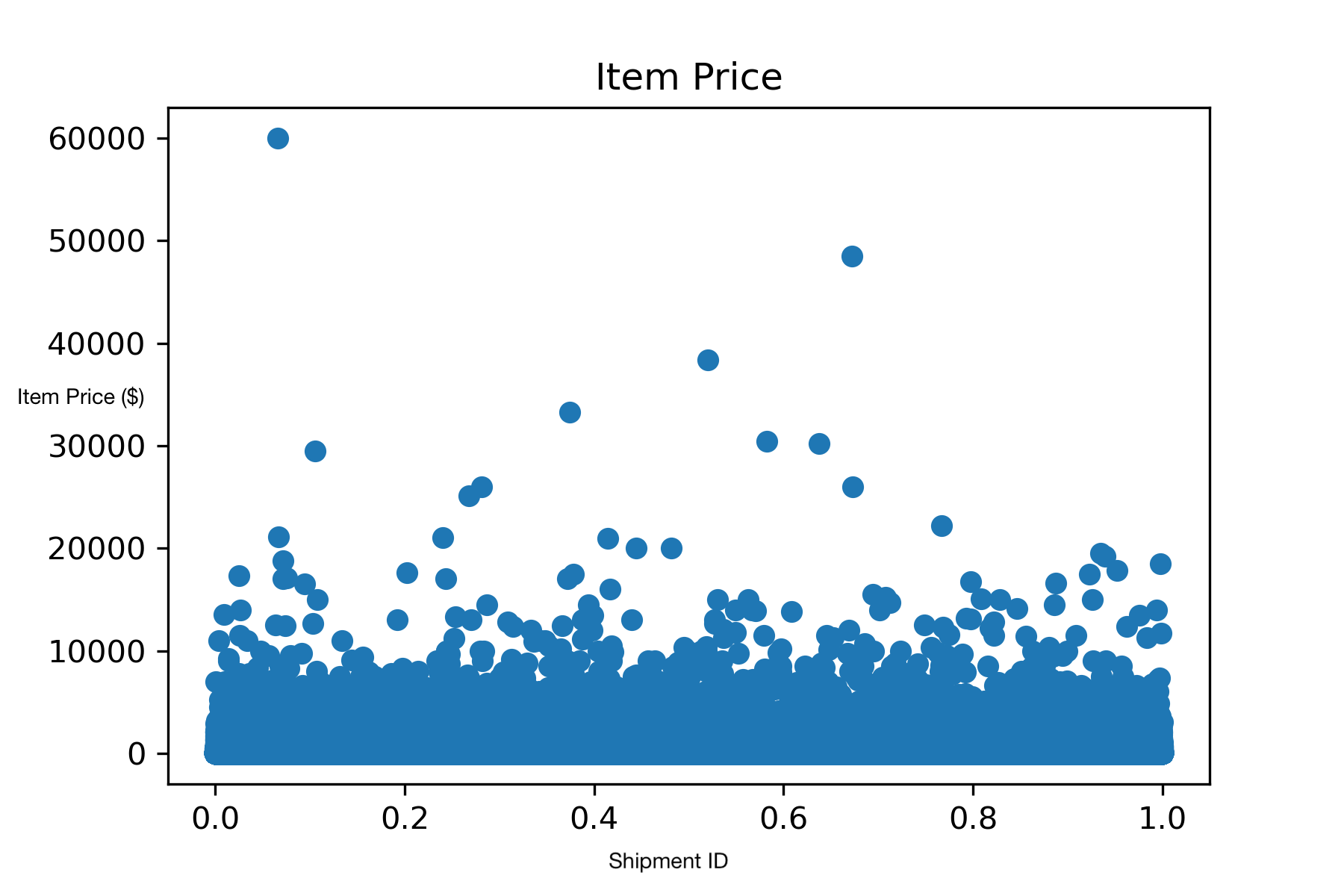
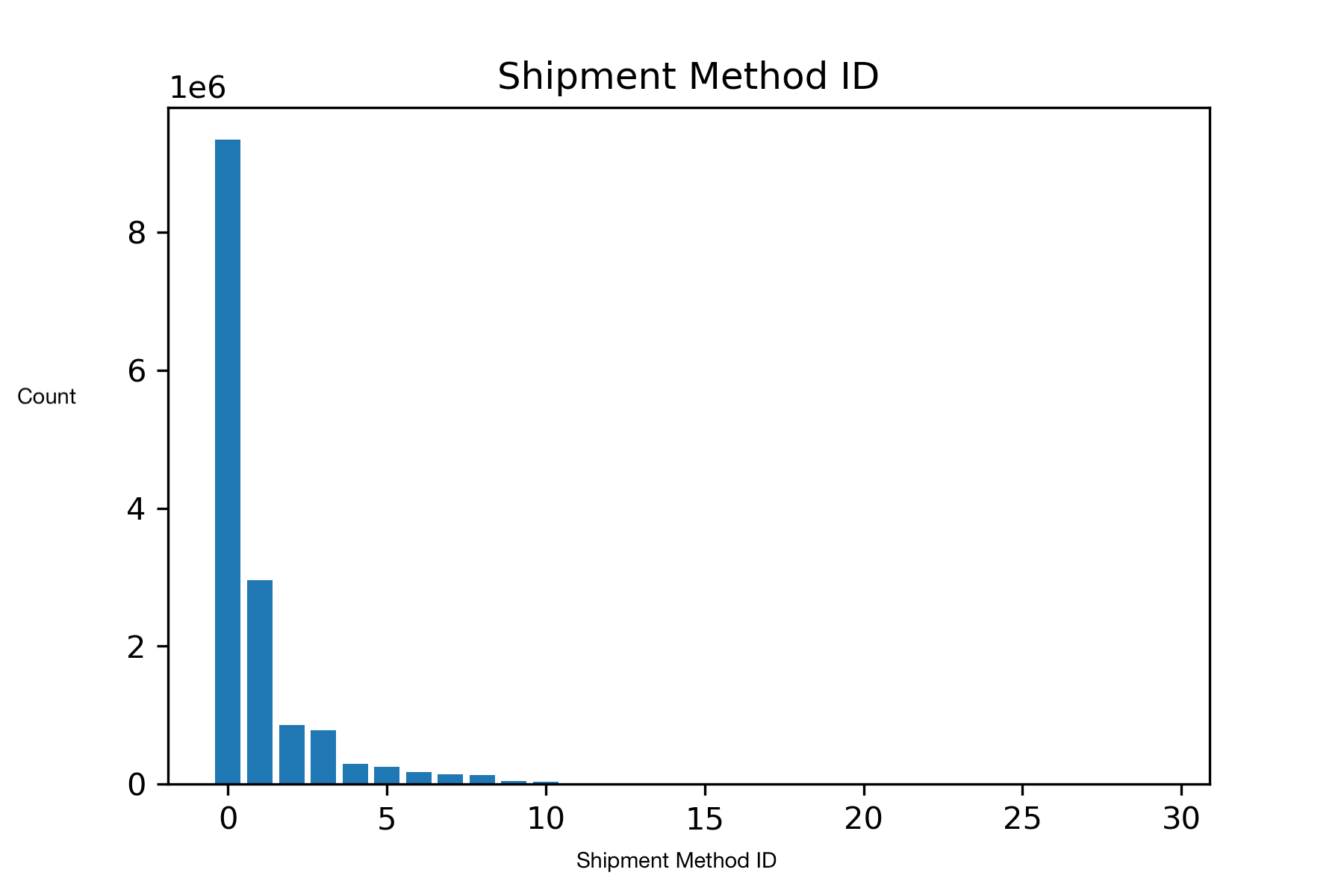
Our dataset was provided by eBay. It contains 15 million shipment records and a validation dataset containing 2.5 million shipment records. Each shipment record contains 19 features. To visualize our dataset, we used the packages pandas and matplotlib. This allowed us to generate graphs for each feature in our dataset. Some of the images we generated include the category ID (which broadly classifies the type of item purchased), the item price, and the shipment method ID (which signifies the type of shipment service declared by the seller to be used for the item).
Goal
Our goal was to use this dataset to create a model that can accurately predict the delivery time (in days) of an eBay shipment. To accomplish this goal, we broke our problem down into a few steps:
- Cleaning our data
- Creating new features
- Determining feature importance
In all of the following models, the word ‘loss’ can be interpreted as the weighted average absolute error of the delivery predictions in days.
Cleaning our data
To clean our dataset, we first needed to handle irregularities and missing data. To do so, we omitted some examples, and replaced other examples with averages from similar training instances. Many of the data points contained missing entries, so to account for this, we either replaced the entries or deleted them.
For example, one of our features, the minimum/maximum transit time that the carrier provided, had many missing entries, so we replaced the missing entries with an estimate that we calculated by obtaining an average transit time based on the shipment_method_id feature associated with that item. We did this for the declared handling days feature as well, using an average from the seller id feature. Finally, we also did this for any missing entries in the weight feature by replacing them with the average weight for shipments that have the same category as the item.
We also had to clean the data so that all entries were able to be used by the neural network. We converted features that were represented as strings, such as b2c_c2c and package_size, into discrete numeric encodings. For b2c_c2c, the original variable format was either ‘B2C’ or ‘C2C’ as strings. We encoded these instead as 0 and 1, respectively. For the package_size variable, the original data was symbolic and in the form of ‘LETTER’, ‘LARGE_ENVELOPE’, etc. We coded these to numeric integer values, in increasing value of the general size of the packages described such that the order of the integers had importance.
We also converted all of the entries in the weight_units feature to the same unit, instead of having a weight feature and a separate unit feature.
Creating new features
Once we had cleaned the data, we also needed to create a new feature that accounts for the zipcode data we were provided with. We created a new feature: zip_distance, using the item_zip and buyer_zip. The feature zip_distance quantifies the haversine distance between the two zip codes (distance across the surface of a sphere). We utilized the package uszipcode to retrieve a latitude and longitude for zip codes in the packages database and a package called mpu to calculate the haversine distance between the two points. For US zip codes that were not in the database and returned NaNs, we temporarily decided to calculate zip_distance as the distance between the middle of the two states involved in the sale.
Feature engineering
Although we created new features that we thought to be important, we wanted to ensure that those features were necessary for the model. To proceed with this process, we looked at feature importance in both a linear model and a decision tree through XGBoost.
In the linear regression model, we analyzed the coefficients assigned to each input variable. The larger the assigned coefficient, the more ‘important’ the input is for determining the output. We additionally ran a lasso regression for this same purpose, hoping to identify any highly unnecessary inputs and remove over-dependency on highly weighted inputs. However, despite scaling our data, we ran into the issue of having all but one feature assigned a zero or zero-like coefficient.
We also used XGBoost to delineate the most important features. The features nearest the top of the tree are more important than those near the bottom. We ran multiple trees with multiple combinations of variables to see which ones repeatedly showed up at the top of the tree, despite being paired with other variables.
Models
After our data was clean, we began trying different models to see what was most effective and gave the best results.
Linear Regression Model
We decided to start with a naive linear regression. Despite knowing that a linear model could probably not correctly learn this large, complex, real-world data set, linear regression is a powerful algorithm that could at least learn relative feature importance. We used two types of linear regression: (1) standard regression without weight decay, and (2) lasso regression (using L2 penalty). Lasso regression has a an L1 weight decay penalty, and thus tends to push irrelevant features’ coefficients to 0. The results of the two linear regression models are as follows:
| Test Set Loss | |
|---|---|
| Standard Linear Regression (SR) | 0.82 |
| Lasso Regression (LR) | 0.89 |
The following table shows the coefficient values learned for each feature in the two regression models:
b2c_c2c |
shipping_fee |
carrier_min_estimate |
carrier_max_estimate |
|
|---|---|---|---|---|
| SR | 0.2635 | 0.0030 | 0.2217 | 0.4032 |
| LR | 0.0 | 0.0 | 0.0 | 0.0 |
category_id |
item_price |
quantity |
weight |
|
|---|---|---|---|---|
| SR | 0.0183 | -0.0001 | 0.003 | -9.5e-06 |
| LR | 0.005 | 0.0001 | 0 | 1.9e-06 |
Standard linear regression suggests that carrier_max_estimate, carrier_min_estimate, and b2c_c2c are the most important features. It also learned that shipping_fee and quantity are of minimal, but non-zero importance. The remainder of the features are found to have no importance. However, these models do not perform well relative to the benchmark random classifier loss provided by eBay: 0.75 (the weighted average absolute error of the delivery predictions in days). The models only performed better than a random classifier by 0.07 and 0.14 respectively.
Fully Connected Model
We additionally created a fully connected model with 7 hidden layers, each activated using ReLU. With eBay’s criterion and the Adam optimizer, the model performed the best with a learning rate of 0.0001 and a batch size of 256.
After 125 epochs over about 11,000,000 training and 3,000,000 validation examples, the model achieved a loss of 0.411 given the input features:
b2c_c2ccarrier_min_estimatecarrier_max_estimateweightzip_distancehandling_days

To tune each hyperparameter, we trained the model on 150,000 examples over 100 epochs multiple times and compared its losses, adjusting only the hyperparameter that was being tuned and holding all others constant.
| Learning Rate | Loss |
|---|---|
| 0.001 | 0.470 |
| 0.0001 | 0.533 |
| 0.00001 | 0.692 |
While the run with a learning rate of 0.001 reached the lowest loss, it oscillated for the last 10 epochs, suggesting it would converge too quickly for the final model which would train over more epochs and on significantly more data per epoch. Conversely, the run with a learning rate of 0.00001 spent its last 10 epochs with a stable loss no greater than 0.693, suggesting it reached a local minimum or simply learned at an extremely slow speed. As a result, we chose a learning rate of 0.0001 as, while its run did not reach the lowest loss, it spent its last 10 epochs steadily decreasing in loss, suggesting it might converge at a lower loss after more epochs and with more data than it would with a higher learning rate.
| Batch Size | Loss |
|---|---|
| 16 | 0.698 |
| 32 | 0.451 |
| 64 | 0.452 |
| 128 | 0.457 |
| 256 | 0.459 |
| 512 | 0.499 |
We initially chose a batch size of 32 as its run reached the lowest loss. However, the resultant model was extremely slow to train on the full dataset at over 2 hours per epoch. Consequently, we chose a batch size of 256 as the loss achieved during its run was only marginally higher than the loss achieved by the run with a batch size of 32, while requiring significantly fewer computations per epoch.
In tuning the architecture, we set a maximum number of neurons in the first hidden layer. The number of neurons in each following layer was half that of the previous until the number of neurons in a layer was 8. For instance, if the number of neurons in the first hidden layer was 64, the following hidden layers would have 32, 16, and then 8 neurons.
| Neurons in First Hidden Layer | Loss |
|---|---|
| 64 | 0.662 |
| 128 | 0.536 |
| 256 | 0.463 |
| 512 | 0.456 |
| 1024 | 0.457 |
We chose an architecture with 512 neurons in the first layer as its run reached the lowest loss.
XGBoost
XGBoost is a popular gradient boosting decision tree algorithm that has been featured in the winning submissions of many machine learning competitions. Essentially, XGBoost is an ensemble method that combines several weak learners (the individual decision trees) into a strong one. Gradients come into play when each new tree is built; subsequent trees are fit using the residual errors made by predecessors. Another advantage of XGBoost is its interpretability. Trees are easy to understand, and they are great models for discerning feature importance. The higher up a feature is on the various decision trees, the more important that feature is. As each tree is built, splits are decided based on what “decision” (i.e. is b2c_c2c true or false?) best evenly partition the data. This is why features high up in the tree are indicators of the most important features. XGBoost performs well on various datasets, and we wanted to explore how it would perform on the eBay dataset.
Feature importances learned by XGBoost:
| Feature | Feature Importance |
|---|---|
b2c_c2c |
0.015656 |
seller_id |
0.047507 |
declared_handling_days |
0.042284 |
shipment_method_id |
0.035131 |
shipping_fee |
0.028294 |
carrier_min_estimate |
0.044301 |
carrier_max_estimate |
0.055198 |
item_zip |
0.059736 |
buyer_zip |
0.028275 |
category_id |
0.022790 |
item_price |
0.042802 |
quantity |
0.047650 |
weight |
0.057305 |
package_size |
0.020258 |
By far the most importance feature learned by XGBoost is handling days, a feature we engineered from the difference in acceptance_carrier_timestamp and payment_date (i.e. the number of days between the time the package was accepted by the shipping carrier and the time that the order was placed). Following this, it seems that weight, item_zip, buyer_zip and carrier_max_estimate are also important. The only features that XGBoost has learned to have lower or minimal importance are buyer_zip_median_incom, item_zip_pop_density, package_size, category_id, buyer_zip, shipping_fee, and b2c_c2c. We can, to some extent, trust that the feature importances learned by XGBoost carry some weight, because the model was able to achieve a loss of 0.50 (the weighted average absolute error of the delivery predictions in days), a large improvement from the linear regression models.
CatBoost
Another tool we used is a random forest/decision tree package called Catboost. This is similar to XGBoost, however it focuses on categorical data (hence the “cat” in Catboost). This is discrete data that represents categories rather than continuous numerical data. This tool was useful to us because several of our important features are categorical, such as zipcodes, package size (small, medium, large), and item type.
Upon a preliminary test of a Catboost model on a subset of our data (20,000 rows) with default parameters, we were able to achieve a loss of 0.49 (the weighted average absolute error of the delivery predictions in days) using the loss function provided by eBay. This is a promising number, considering the small subset of data used and lack of fine tuning. The contrast of Catboost’s performance shows how a categorically tailored package seems to be a better choice. Catboost also includes an overfitting-detection tool. This stops more trees from being created if the model begins to perform worse.
According to Catboost documentation, the best parameters to fine tune are: learning rate, L2 regularization (coefficient of the L2 regularization term of the cost function), and depth (the number of trees created). After testing a variety of values for these parameters, we found that a learning rate of 0.375, a L2 regularization coefficient of 5, and a depth of 8 yielded the lowest loss. We then moved forward with these parameters.
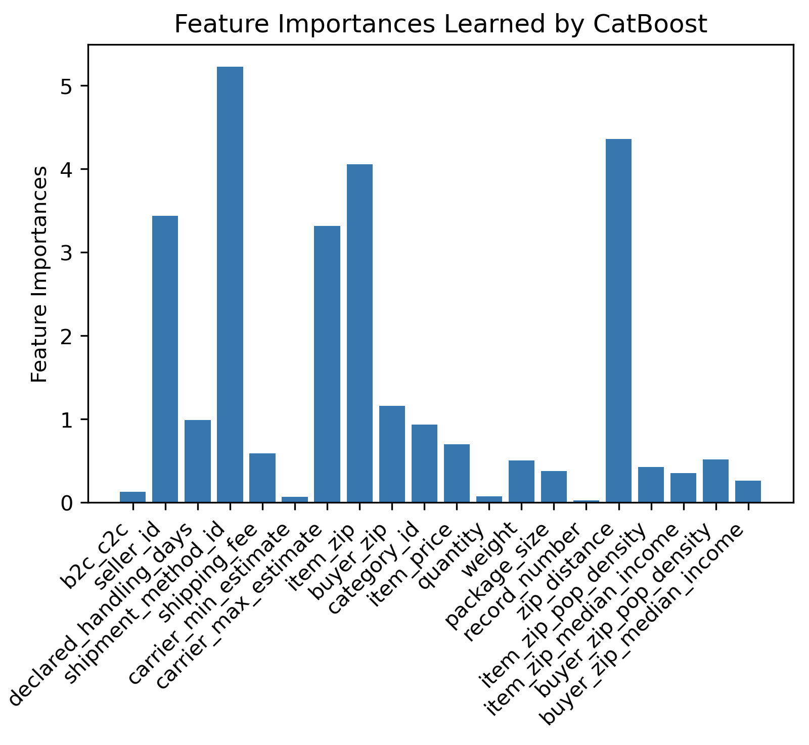
Ultimately, after tuning hyperparameters and running Catboost on all of our data (15 million rows), we were able to achieve a loss of 0.453. The feature importances of this model can be seen in the table below. Handling days was clearly the most important; this is a feature we engineered which is the difference in days between the acceptance_carrier_timestamp and payment_date. This makes sense, as it represents the speed at which the seller shipped the package.
Feature importances learned by Catboost:
| Feature | Feature Importance |
|---|---|
b2c_c2c |
0.129 |
seller_id |
3.44 |
declared_handling_days |
0.993 |
shipment_method_id |
5.32 |
shipping_fee |
0.591 |
carrier_min_estimate |
0.07 |
carrier_max_estimate |
3.32 |
item_zip |
4.06 |
buyer_zip |
1.16 |
category_id |
0.938 |
item_price |
0.701 |
quantity |
0.075 |
weight |
0.503 |
package_size |
0.380 |
record_number |
0.267 |
zip_distance |
4.36 |
item_zip_pop_density |
0.426 |
item_zip_median_income |
0.352 |
buyer_zip_pop_density |
0.518 |
buyer_zip_median_income |
0.266 |
handling_days |
72.1 |
Loss function
After training our models, we used the loss function provided by eBay of which the baseline (random guessing) loss is 0.759 (the weighted average absolute error of the delivery predictions in days). This loss function is essentially an average of how many days the prediction was off by, where late predictions are weighted more heavily than early predictions. Our goal was to obtain a loss that is significantly lower than 0.759 for our model.
Models
Once we had cleaned and processed our data, we trained 4 models to compare the results from each one. These models were:
- Linear regression
- Fully connected neural network
- XGBoost (decision tree gradient boosting algorithm)
- CatBoost (another decision tree gradient boosting algorithm that deals better with categorical features)
Results
Comparing the results of the models, the fully connected model performed the best.
| Model | Loss |
|---|---|
| Linear Regression Model | 0.82 |
| Fully Connected Neural Network | 0.411 |
| XGBoost | 0.50 |
| CatBoost | 0.453 |
The resulting quantity loss can be called the (average) loss, the penalty, or the score. Lower loss scores represent better models. It signifies that the model predicts shipping days better according to eBay’s loss function, which takes into account whether the model predicted the shipping days to be greater than or fewer than the real shipping days. A greater penalty was placed when models incorrectly predicted the shipping days early, since that renders more customer dissatisfaction.
Discussion
Model Evaluation: Feature Importance
To evaluate our models, we first looked at the features that the models deemed to be the most important. We were able to gather this information for XGBoost and CatBoost. We did this so we could determine whether the models performed well on certain subsets of the data, analyzing whether some subsets had bias, or if XGboost and CatBoost prioritized certain features over others.
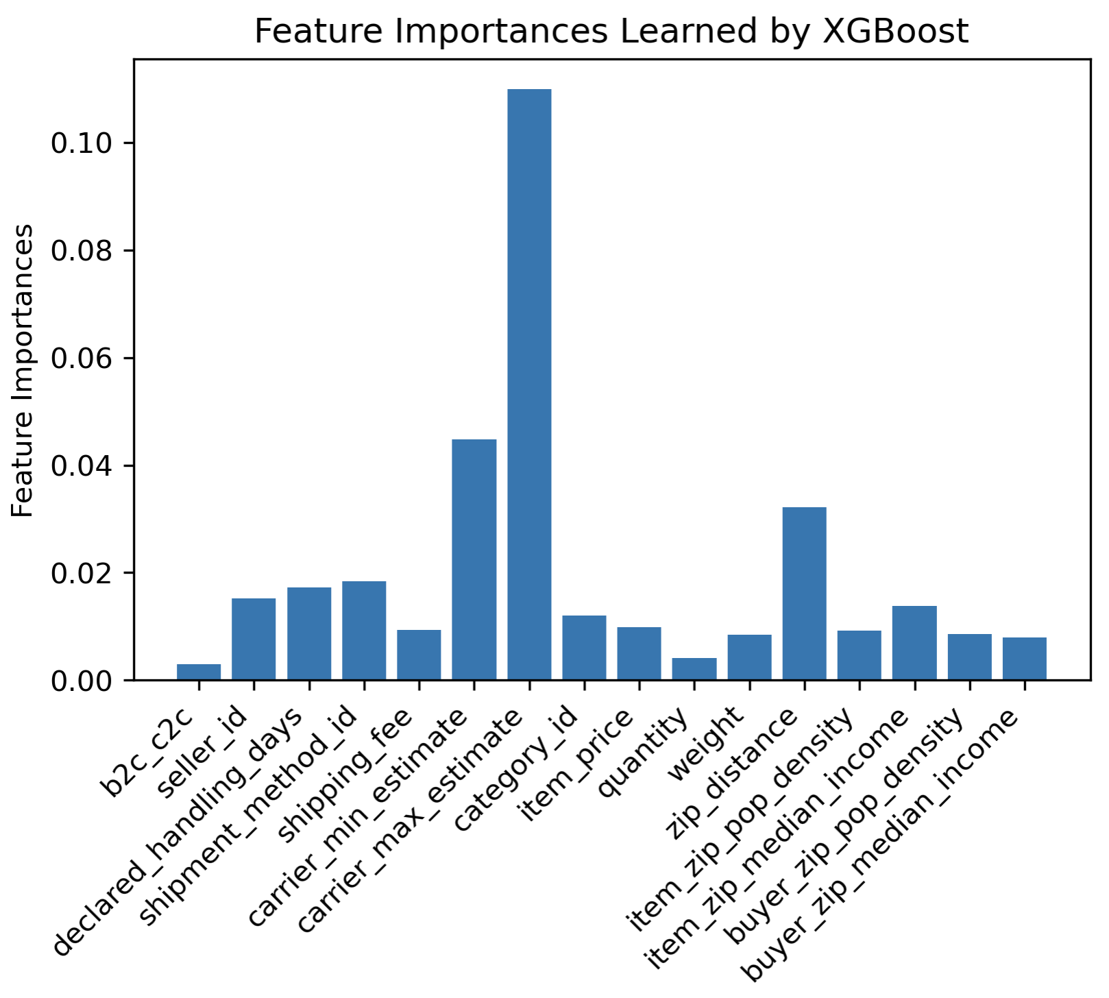
XGBoost learned many boosted decision trees on random subsets of the data. Features that are evaluated higher up in the trees correspond to the features which the model has learned are more important. We have found that the most important features are handling_days and carrier_max_estimate, followed by some mid-tier importance features such as weight, zip_distance, and shipment_method_id.
CatBoost was able to identify a larger set of importance features, which include seller_id, shipment_method_id, carrier_max_estimate, item_zip, and zip_distance. It makes sense that CatBoost was able to learn the importance of seller_id, shipment_method_id, and item_zip because these are categorical features. This was exactly our motivation for using CatBoost, so this indicates that was a good decision.
In these graphs, we removed the handling_days feature that we engineered, but XGBoost and CatBoost both learned that it was by far the most important feature. We engineered this feature by calculating the difference in days between the time the carrier accepted the package from the seller and the time the order was placed. Because the magnitude of importance was so much higher, it made these bar graphs uninterpretable, so we have simply removed that feature from the graph.
Model Evaluation: Predictions
We also wanted to compare how the models might differ in effectiveness. To do so, we can look at the loss by each model compared visually to each other as well as the eBay benchmark.
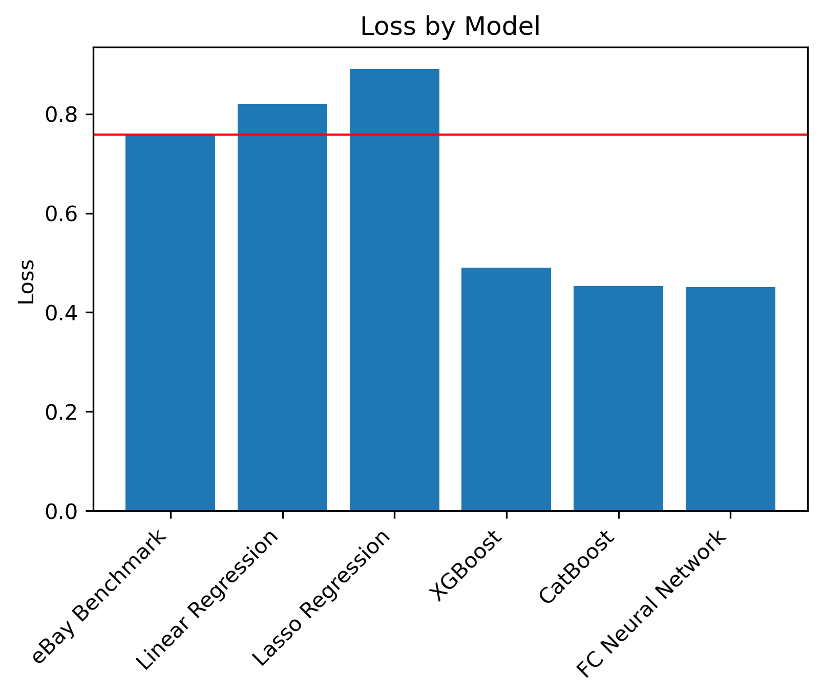
In this graph, we compare the losses of each model and also look at eBay’s benchmark, which is represented by the red line. We included the benchmark because it can help us visualize whether the models made meaningful predictions (better than a random guess). We can see that CatBoost and the Fully Connected Neural Network performed the best, and XGBoost was also effective as a close third option.
Our dataset has many categorical features, like shipment_method_id, item_zip, buyer_zip, and b2c_c2c. XGBoost and CatBoost performed relatively well, which motivated using a similar algorithm that could better handle these categorical features. We also fine-tuned our Fully Connected Model and found that our fine tuning improved the model considerably. We believe this is the main reason why our FC NN had the best performance.
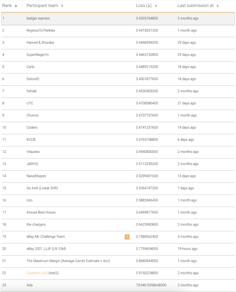
Comparison
To compare our work with others, we used the leaderboard of losses from other teams participating in the competition. However, it should be noted that the leaderboard may not currently represent the results of the most recent models as the competition does not end for another month and teams may withhold from posting their losses until then.
Currently, our model holds a 0.023 loss lead.
Ethics Discussion
One of the key implications of fast shipping is the effect that it has on the environment. The environmental effects of shipping are widespread, affecting everything from air pollution and water pollution to oil spills and excess waste. The increase of fast delivery times and same-day delivery options provided by companies has led to a greater environmental cost such as more trucks on the road, air quality issues, and package waste. Furthermore, there is also a high human labor cost associated with delivery and shipment. The delivery drivers who are responsible for delivering packages to the correct recipients face long shifts without stops, and some companies even encourage fewer stops to prioritize fast shipping. This can lead to detrimental effects as delivery drivers may be incentivized or even forced to provide fast delivery no matter the impact on their wellbeing. It is incredibly important to consider the human impact of fast shipping and prioritize the safety of those who work in the shipping industry. If eBay were to implement a shipment prediction algorithm, it would be incredibly important to ensure that the model was not predicting shipping times that are too fast, or else it may lead to a greater environmental and human impact. Finally, there is a positive impact of shopping on eBay compared to other alternatives (such as Amazon). eBay offers many second-hand goods and products, so consumers buying second hand are positively contributing to the environment by creating less waste. By offering pre-owned items, eBay saves items from ending up in the landfill and promotes sustainable shopping.
Regarding our model specifically, if it were to become deployed we would have to be concerned about a few things. Notably, if our model is wrong and mispredicts delivery times to be way earlier than they actually can be delivered, the actual delivery workers might get wrongfully punished for not meeting the predicted time. It is important to consider how the functionality of our model could impact those who are historically less empowered, including wage workers.
Reflection
This project illustrated to us the difficulty of working with large datasets and the many complexities that come with them. Although the data set was already created for us to use, it was still difficult to clean the data and identify the most important features. When we were cleaning, we decided on replacing missing values with averages, however looking back on our cleaning process, this may have added a lot of noise to our model and hindered accurate predictions. An alternative to this would be to discard missing entries altogether. Next time, we would have tried this instead of using averages to see if it helps our predictions.
To extend this work, we would try to use a tabular model such as fast.ai Tabular. Because our data was in a tabular format, this model may be better suited for the specific kind of data we are using. We could also extend our work by implementing some of the newer algorithms that we read about through our literature review. For example, Wu, F., and Wu, L., (2019) created DeepETA, a new model that works well on time-estimation problems. We would take this model and adapt it for our problem to see if it applies in the case of delivery time estimation.